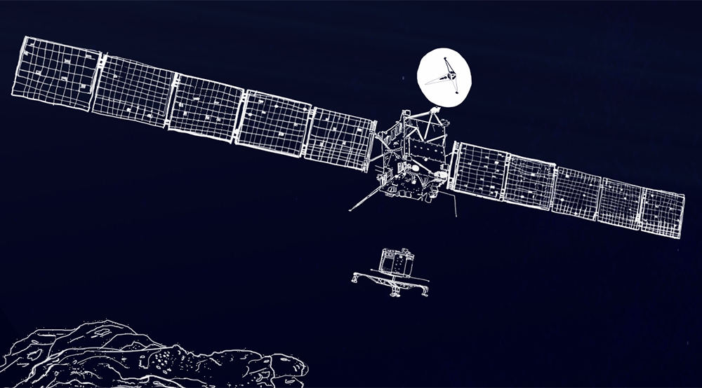
On 5 September 2016 one of the most frequently asked questions among Rosetta mission fans – “Where is Philae?” – was finally answered: the definitive image had been taken just a few days earlier that proved without a shadow of a doubt the location of Rosetta’s lander on the surface of Comet 67P/Churyumov-Gerasimenko. Of course, it wasn’t a chance finding: the clues had been there since Philae bounced out of sight on that thrilling day in November 2014, but it took time and patience – and just a little bit of luck – to finally capture the winning shot. ESA’s Laurence O’Rourke, who led the search campaign in recent months, tells the story of how we found Philae.
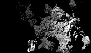
“Welcome to a comet” – Philae’s view of Abydos. Credits: ESA/Rosetta/Philae/CIVA
Playing detective to seek out Philae’s hiding place took more than just viewing Rosetta’s images that had been taken from orbit – it required following many lines of investigation, and the collaboration of many different teams. This included radar data from the CONSERT experiment on both the orbiter and the lander, which was used to help triangulate Philae’s location to the general area; ground-truth images taken by Philae’s CIVA camera to help identify key features of the local terrain; the communication radio frequency (RF) links established between Rosetta and Philae during the lander’s ‘awake’ periods, and the Sun illumination data received from Philae’s solar panels, which together yielded important “line-of-sight” information because in order to see the Sun or Rosetta at certain times there had to be no obstacles blocking the view between Philae and Rosetta or Philae and the Sun. Last but certainly not least, there was also one very promising candidate already proposed by P. Lamy & G. Faury (Laboratoire d’Astrophysique de Marseille), as identified in images taken in December 2014, and published in the blog post The quest to find Philae on 11 June 2015.

Philae’s location marked on a shape model with the previous CONSERT predictions indicated. Credits: Ellipse: ESA/Rosetta/Philae/CONSERT; Shape model: ESA/Rosetta/MPS for OSIRIS Team MPS/UPD/LAM/IAA/SSO/INTA/UPM/DASP/IDA
It is from where that blog post ends that this story really begins. In that post, there were two statements, which seem like premonitions of what was to follow in the search. The first was that “the possibility of further refining Philae’s location would come if the lander were to receive enough power to wake up from its hibernation and resume its scientific study of 67P/C-G. Then, CONSERT could be used to perform additional ranging measurements and significantly reduce the uncertainties on the lander’s location.”
Little did we know that the lander was already awake since late April 2015 and was to send its first signal to Rosetta only three days after that blog post was released! Exciting times indeed and a busy few weeks followed as steps were immediately taken to adapt the trajectory flown to match the line-of-sight between Rosetta and Philae. (The result of the contacts established from then until its last one on 9 July are described in the blog post “Understanding Philae’s wake-up…”. ) Unfortunately the attempt to establish contact via the CONSERT radar was unsuccessful but, even still, the RF contacts we obtained during those few weeks did in fact help us to conclude that the lander had not moved in its location on the surface – a vital input needed in support of the search.
The second statement was that “ultimately, a definitive identification of this or any other candidate as being Philae will require higher-resolution imaging, in turn meaning closer flybys….at significantly less than 20 km from the surface.”
This indeed was very true, but because of the increased activity around the comet’s perihelion in August 2015, Rosetta had to keep at safe distances from the nucleus and it would be March 2016 before we reached 20 km again…
March 2016: Kicking off the lander search campaign…again
When the comet’s activity finally granted Rosetta safe passage to within 20 km of the nucleus again, we kicked off a new search campaign. This was driven by the strong desire of the Lander Steering Committee, the Lander Lead Scientists and the various Philae science and operations teams that ESA should make every effort to identify Philae’s location before the end of Rosetta’s mission, not just for the purpose of knowing where it was, but in order to provide vital context to the scientific data collected by the lander in November 2014. The campaign was led by ESA and involved ESA’s Rosetta Mission Operations Centre (MOC) and Science Ground Segment (SGS) the OSIRIS instrument team, DLR’s Lander Control Center, and CNES’ Philae Science Operations and Navigation Center (SONC) teams.

Context image showing the relative positions of the ‘red’ and ‘blue’ candidates. The image was taken on 9 March 2016, 15 km from the surface. Credits: ESA/Rosetta/MPS for OSIRIS Team MPS/UPD/LAM/IAA/SSO/INTA/UPM/DASP/IDA
The campaign was primarily focused upon imaging two possible lander candidates, which we identified simply as the red and blue candidates (see image above). Red corresponded to the Lamy & Faury candidate, which not only lay within the CONSERT ellipse and appeared to meet the various power, RF and visibility constraints linked to the actual data from the lander, but also showed promising correlation between CIVA and OSIRIS images. The blue candidate was located further south however, and could only really be deemed possible if the lander had in fact moved during the perihelion passage.
But even with these two candidates we still could not discard the possibility that the actual lander might be in a different location, albeit most likely within the CONSERT ellipse. Following a proposal from P. Muñoz of ESA’s MOC Flight Dynamics team, the campaign was performed with the strategy to take images within this ellipse from different viewing angles around the comet. This addressed two issues: the first being that the lander might be blocked by a rock from one direction while visible from another, and the second being that such an approach allowed different illumination conditions and phase angles to be taken into account.
The devil is in the detail: those involved in image planning and analysis
Once the trajectory to be flown by Rosetta for its primary science mission was fixed by the flight dynamics team, it was then analysed by the lander search team members to identify the possible times where there would be line-of-sight visibility between Rosetta and the Philae candidates, and whether it would be well-illuminated. (The provision of the visibility windows for the March – June timeframe was made by MOC Flight Dynamics (P. Muñoz) and CNES SONC Flight Dynamics teams (E. Jurado, R. Garmier, A. Charpentier); the windows for July–September were provided by B. Geiger on the Rosetta SGS side. Analysis plots as shown in Figure 3 were provided by CNES/ SONC, by MOC Flight Dynamics (P. Muñoz) and by B. Grieger of the SGS).

Two different ways of viewing the orbiter flight trajectory when compared to the lander position. Left: how Rosetta’s trajectory (in blue) appears over the horizon in terms of Philae’s antenna field-of-view. Green markers indicate the contact locations where Philae had a direct line of sight with Rosetta to communicate in November 2014 and June/July 2015. Right: The lander position is in the centre and the figure shows the local horizon scaled with the co-elevation in degrees. For example, if Rosetta flies directly over the centre point then the lander will be directly below Rosetta. The further Rosetta flies towards the edge of the plot, the closer to the horizon it will be. Rosetta’s trajectory is again shown in blue with lines linked to the track of the Sun across that point during the same time. The equivalent RF link (green) and Philae illumination lines (yellow) are shown on the plot to show where Rosetta should fly to mimic the line-of-sight conditions that Rosetta and Philae shared during contact. Credits: left: CNES/SONC/Flight Dynamics; Right: ESA/Rosetta/MOC/P.Muñoz.
The choice of which trajectories should actually be flown were based upon factors such as minimising impact on key orbiter science observations planned during those periods, avoiding times where the orbiter/Sun was below 20º from the horizon, avoiding spacecraft manoeuvres, and avoiding times where the spacecraft pointing error was predicted to be high (more about this later). As the lander campaign progressed and we obtained a clearer idea of the local topography blocking our view, so the selection of windows became more refined. Similarly, as Rosetta’s trajectory became fixed in preparation for the end of mission descent, this placed a lot of constraints on the remaining windows feasible during August and early September (more about this later, too).
When a window had been selected, there were three steps to be taken: ensure the pointing of the spacecraft was updated so that it would point exactly at the location of a lander candidate (this was done by members of the MOC Flight Dynamics group (C. Bielsa) for certain windows and by the Rosetta SGS (R. Andres, RSGS operations & planning group) for others); prepare the commands to be sent to the OSIRIS cameras for the time period in questions (this was performed by OSIRIS team members (P. Gutierrez-Marques, C. Tubiana, C. Guettler, J. Deller, Principal Investigator H. Sierks); and finally sending these commands via the SGS to the MOC flight control team (led by S. Lodiot), at which point they were uploaded to the spacecraft for execution on board.
When the data was downlinked, analysis of the images was performed in parallel by the lander search team including members from the OSIRIS team (C. Tubiana, C. Guettler, H. Sierks), from the SGS (myself) and from the SONC team (J. Durand, A. Charpentier, G. Faury).
When is close not close enough?
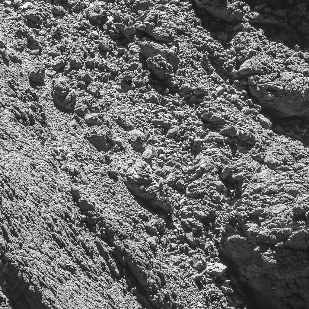
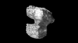
The animated gif below shows an image taken at a distance of about 18 km from the comet on 5 March 2016, which targeted the region around the red candidate, and which really illustrates the challenges presented by the local scenery. There are the two major features that surround the red candidate: a ‘cliff overhang’, and a large ice/dust structure that has a slightly triangular shape, which we nicknamed the ‘nose rock’. In addition, the edge of the Hatmehit depression is also close by.
The scenery around Philae includes a ‘cliff overhang’ and a large ice/dust structure nicknamed the ‘nose rock’ (labelled). An enhanced view of the same region is shown, with a circle highlighting the lander candidate that becomes visible in the darkness from the reflected light emanating from the outside of the cliff. The last image shows the orientation of the lander from the 3D model. Credits: Image: ESA/Rosetta/MPS for OSIRIS Team MPS/UPD/LAM/IAA/SSO/INTA/UPM/DASP/IDA: Lander search analysis: L. O’Rourke; CNES/GFI/3DView tool/J. Durand/ G. Faury
The impact of these features on the ability to image the red candidate is better seen in the animated gif below. This lander candidate is basically located between a rock and a hard place 🙂
The challenges of trying to get the right perspective, taking into account illumination and local topography constraints such as the ‘nose rock’ or the edge of the Hatmehit ‘crater’. Credits: Images: ESA/Rosetta/MPS for OSIRIS Team MPS/UPD/LAM/IAA/SSO/INTA/UPM/DASP/IDA; Lander search analysis: L. O’Rourke
At a distance of 18 km, the images yield a scale of ~ 36 cm per pixel so the lander would only be around three pixels across. To identify the lander at this distance proved to be very difficult. Even a few kilometres closer at 15 km (such as the second image shown in this post), the lander appears as a bright point: the resolution was far from sufficient to make a clear identification. It was at this stage that the lander search team decided to only take images of the lander candidates below a distance of 10 km.
The blue candidate is discarded thanks to an image taken on 21 July 2016 that shows it to be ice. Credits: Images: ESA/Rosetta/MPS for OSIRIS Team MPS/UPD/LAM/IAA/SSO/INTA/UPM/DASP/IDA; Lander search analysis: L. O’Rourke
All that glitters is not gold: discarding imposter landers
As we got closer to the comet the image resolution improved, giving us better views of the red and blue candidates but also unfortunately leading to new lander candidates being found in the region of interest! A high resolution image taken on 21 July finally allowed us to discard the blue candidate – it turned out to be ice on the edge of a large boulder (above). We had to study many new images from different perspectives to discard the other ‘fake Philaes’ – see below for examples of some of the more convincing imposters!
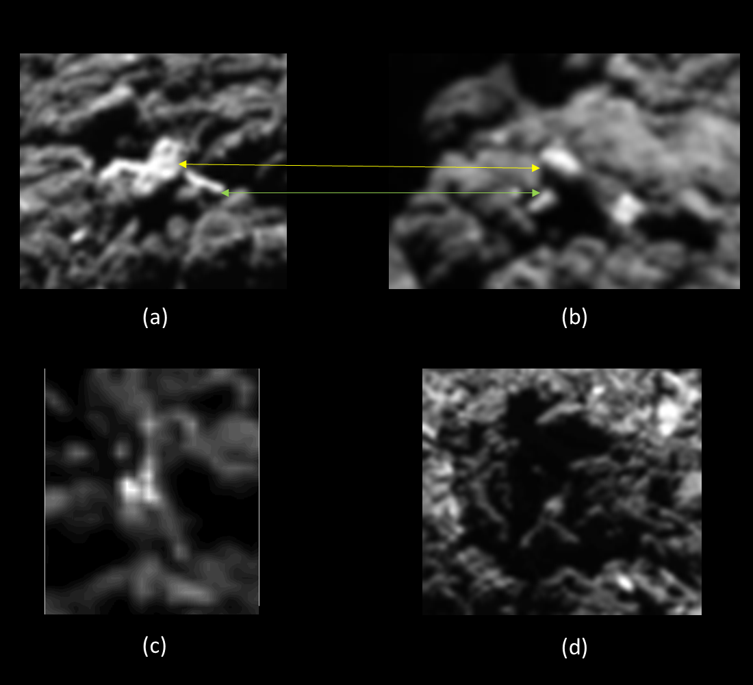
Imposter landers. (a) and (b) show the front and overhead view of one of the lander imposters: a change in orientation from (a) to (b) reveals its true nature as an icy boulder. Images (c) and (d) also both show ice on the front of a boulder giving a lander-like impression at first glance.
Credits: Images: ESA/Rosetta/MPS for OSIRIS Team MPS/UPD/LAM/IAA/SSO/INTA/UPM/DASP/IDA; Lander search analysis: L. O’Rourke
In the meantime, the case continued to build for the red candidate. On 25 May we looked over the edge of the nose rock into the cliff cavity and there we saw what appeared to be a lander-like structure including a leg and foot (image below). We saw something similar on 1 June and also on 6 August from a different perspective and altitude, as seen in the following images:
Images taken on 25 May 2016, with key landscape features labelled and the lander candidate circled. A 3D view of Philae is included for comparison. Credits: image: ESA/Rosetta/MPS for OSIRIS Team MPS/UPD/LAM/IAA/SSO/INTA/UPM/DASP/IDA; Lander search analysis: L. O’Rourke; 3D Philae shape: CNES/ A.Charpentier
![[Fig 9]: Image taken on 01 June 2016 with 3D view of Philae at same time for comparison purposes. Credits: images: ESA/Rosetta/MPS for OSIRIS Team MPS/UPD/LAM/IAA/SSO/INTA/UPM/DASP/IDA; 3D Philae shape: CNES/ A.Charpentier; Lander search analysis: L. O’Rourke](https://blogs.esa.int/rosetta/files/2016/09/Figure-9-Lander-June-1st.png)
Image taken on 01 June 2016 with 3D view of Philae. Credits: images: ESA/Rosetta/MPS for OSIRIS Team MPS/UPD/LAM/IAA/SSO/INTA/UPM/DASP/IDA; 3D Philae shape: CNES/ A.Charpentier; Lander search analysis: L. O’Rourke
Images taken on 6 August 2016 shown with key landscape features labelled and the lander candidate circled. A 3D view of Philae is included for comparison. Credits: Images: ESA/Rosetta/MPS for OSIRIS Team MPS/UPD/LAM/IAA/SSO/INTA/UPM/DASP/IDA; 3D Philae shape: CNES/ A. Charpentier; Lander search analysis: L. O’Rourke
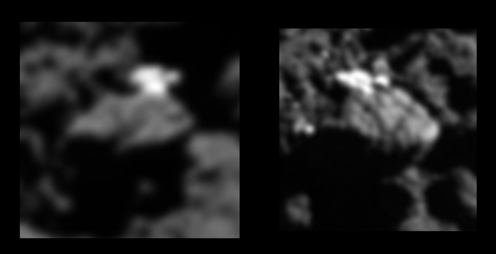
However, within these images there exist not only bright reflective surfaces that could be those of the lander but, unfortunately, also could be due to icy ‘lines’ and patches weaving through the cliff overhang. An example of these features are shown for two 25 May images below.

Two different images taken on 25 May 2016 with similar “ice” features highlighted as those of the reflected parts of the red candidate. Credits: images: ESA/Rosetta/MPS for OSIRIS Team MPS/UPD/LAM/IAA/SSO/INTA/UPM/DASP/IDA; Lander search analysis: L. O’Rourke.
Taking this into account, as well the fact that the resolution was still not sufficient to make a 100% convincing claim that this was Philae, we continued to build our case using evidence from our parallel investigative studies.
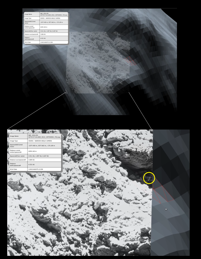
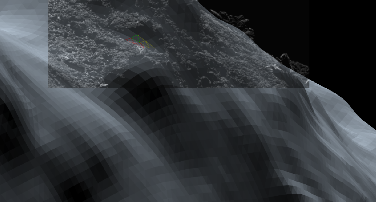
Checking OSIRIS images (foreground inset) against 3D shape models (background). The triangular facets helped identify the location visibility. This approach is used in planning the observations as well as in checking the results afterwards. Credits: ESA/Rosetta/SGS/R. Andres; Inset: ESA/Rosetta/MPS for OSIRIS Team MPS/UPD/LAM/IAA/SSO/INTA/UPM/DASP/IDA
The pieces of the puzzle come together
While the focus of the campaign based itself around the use of direct image visual analysis, other key techniques and resources were being used to support the search. This included:
- Checking the best pointing and visibility opportunities against 3D shape models (see image right)
- Checking OSIRIS images against high-resolution 3D shape models (see image right)
- Updating the local Digital Terrain Model of the CONSERT ellipse region to allow a better comparisons to be made, including reconstructing the view of the CIVA images (this work is in preparation as a science paper to be published in the coming months).
- Comparing the CIVA images against the high resolution OSIRIS images taken at the different lander candidate locations to look for correlations (this work is also in preparation as a science paper to be published in the coming months).
- Comparing RF and power illumination visibility periods with the different lander candidates to see which ones best fit the actual data e.g. Blue candidate (see image below)
- Constructing a map of the locations around the red candidate where it was visible and not visible in the imagery, to compare with the real RF and Sun illumination data from lander contacts (see image below). For example, in image (c) below there was a very clear correlation demonstrated between the location in the trajectory from where RF signal was received versus the Rosetta (OSIRIS)/sun visibility of the red candidate.
- Kicking off a study to perform computer based automatic analysis of images to identify lander candidates: this was performed by CNES in 2015 and also addressed by an ESA-led study this year.
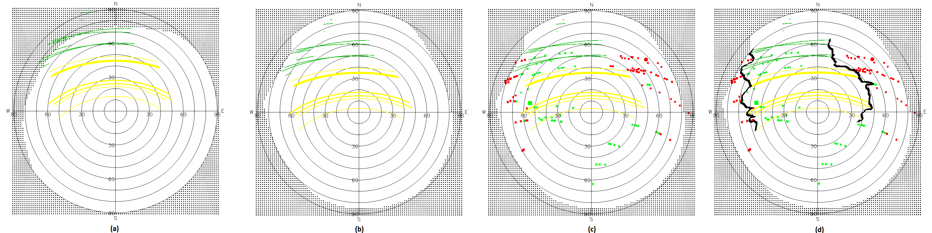
Rosetta-Philae line-of-sight maps, for the blue (a) and red (b-d) candidate. Green lines indicate RF visibility during actual lander contacts, yellow lines are Sun illumination measured by the Philae lander. (a) shows that from this blue candidate position not all contacts were possible so the lander would need to have moved to reproduce this result. (b) RF and Sun illumination lines for the actual Philae “red” candidate. (c) The trajectory locations where the Philae “red” candidate was actually seen in OSIRIS images (with squares being Rosetta viewpoint and circles the sun illumination status) over-plotted on (b): one can see there is a very good correlation between positions where Philae is not visible from Sun or Rosetta and the positions from where no RF signal was obtained thus providing strong evidence for this candidate being Philae (d) The same plot as (c) but this time with a horizon mask drawn to show what topographical features blocked the view. Credits: ESA/Rosetta/SGS/B. Grieger/ B. Geiger/L. O’Rourke; Lander search analysis: L. O’Rourke
With this combined evidence pointing more and more towards the red candidate being the true Philae lander, we decided to schedule more OSIRIS images to be taken in late August to attempt to see the “ice legs” previously seen in May-August images ‘move’ against the background terrain, by viewing it from different angles. This would confirm the structure there was indeed a human-made object rather than ice.
So close and yet so far
As Rosetta gradually began getting closer to the comet in August and early September, and with the mission end just weeks away, the number of opportunities to get images of the red candidate were diminishing fast – and not just because of time constraints. For starters, the lander visibility windows were taking place in the orbit when the red candidate was now always in darkness. To offset this, we tried to schedule the images to be taken as late as possible in the slot to improve the reflected light coming from the outside of the cliff. In addition, the OSIRIS team members performed their magic to take advantage of the wide dynamic range of the camera and take images trying to capture as much light as possible. This was tested very well and was implemented for the late August windows.
Another tricky factor was trying to image over the nose rock into the cavity where the candidate was located. In August through to September, the trajectory was such that we were gradually moving north with respect to the lander position. Having spent quite some time looking at the images during the months of the search, it became clear to me that the 3D shape model was not a perfect tool for scheduling these images because it assumed the edge of the nose rock to be smooth and straight, when in reality it is far from that. I had seen gaps in the leading edge of the rock: if we were to take an image from a certain angle we could surely see areas that would normally be blocked –and defined by the shape model to be blocked – by the nose rock. Similarly, the topography of the starting edge of the nose rock also had some discrepancies with the shape model (see image below).
An overlay of an OSIRIS image of the nose rock on the 3D shape model where the discrepancy between the two is clear. Credits: ESA/Rosetta/SGS/R. Andres; Inset: ESA/Rosetta/MPS for OSIRIS Team MPS/UPD/LAM/IAA/SSO/INTA/UPM/DASP/IDA
The lander search campaign was due to end in fact on 30 August with the general view that the offending ‘rock’ would block the view, as it had done for images attempted on 21 and 24 August. However, I was still certain that with the right angle, the lander candidate would be visible. As a result, I proceeded to convince the mission manager (P. Martin), Project Scientist (M. Taylor) and the lander search team to schedule further images for 2 and 5 September on the basis that as we moved along the lower edge of the nose rock we would finally reach a point where we could see over its irregular edge. Thankfully my insistence won through!
Saving the best ‘til last
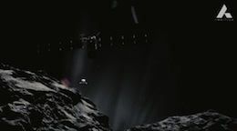
On 2 September, Rosetta’s field of view allowed us to look over the very front edge of the nose rock at a distance of 2.7 km from the surface, and take high-resolution images – 5 cm/pixel. When the images were downlinked to Earth on 4 September, the first to see them was Cecilia Tubiana from the OSIRIS team. She studied the images and searched for the red candidate in the position under the cliff where we had pointed the spacecraft, and there it was: hiding in the corner of the image.
Philae was spotted on the far right hand side of an image taken on 2 September 2016. Credits: ESA/Rosetta/MPS for OSIRIS Team MPS/UPD/LAM/IAA/SSO/INTA/UPM/DASP/IDA
After some 22 months since it landed, and with the comet, Philae and Rosetta at a distance of approximately 680 million kilometres from the Earth, the location of the Philae lander was known at last. The lower resolution images taken previously, which had hinted at a lander-like structure, could finally be confirmed retrospectively as Philae. The red candidate, originally proposed by Lamy & Faury back in 2015, was at last confirmed to be the Philae.
Animated GIF of Philae as observed on 2 September 2016 compared with the 3D model. Credits: 3D Philae shape: CNES/A.Charpentier; inset : ESA/Rosetta/MPS for OSIRIS Team MPS/UPD/LAM/IAA/SSO/INTA/UPM/DASP/IDA
Moreover, Philae was inside the CONSERT radar triangulation result and its attitude close to that derived by the Philae Lander team. The image also proved that the lander cannot have moved significantly since it landed at Abydos in November 2014.
This confirmed position provides the much sought after context needed to better interpret Philae’s science measurements made in November 2014 (a summary of the exceptional science already published by the Philae science teams can be read here).
A near miss
But there was one final factor at play that nearly made this now-famous image another miss. You may have noticed that instead of the lander being nicely framed in the centre of the image, which was our plan, it is skewed all the way over on the right hand side. For this “off-pointing” we can primarily blame the comet. Due to the close distances of our flyovers, the trajectory of the spacecraft is affected by the higher gravity drag and cometary gas existing at low altitudes along with normal manoeuvre uncertainties. To overcome this and in order to point the instruments to the Philae location the MOC Flight Dynamics team needed to predict very accurately the spacecraft position with respect to the comet for the whole commanded period. In the case of the 2 September Philae image, this trajectory prediction was performed more than 36 hours before the image was taken achieving an accuracy of ~50 m at the time of the image. So while Philae ended up not being in the centre of the image, the fact that Philae was in the camera field of view at all and not tens of degrees away, reflects the excellent performance of the Flight Dynamics navigation team.
And what of the 5 September image slot? You guessed it: again off-pointing, but in this case the navigation error was much greater than the 2 September slot due to the even closer flyover distance so Philae was completely outside the OSIRIS NAC field of view.
So that image of 2 September, showing the lander in all its glory on the surface of the comet was in fact the last successful image of Philae at Abydos before Rosetta concluded its mission. What a great way to end our search campaign: excitement to the very last image.
Now, after many months of intense work, the lander search group is winding up its activities. There is no doubt that without the significant work, drive and efforts of all teams and individuals involved in the lander search group (only some of whom have been mentioned in this article), the lander would not have been imaged before Rosetta itself makes its own touchdown on the surface of the comet on 30 September.


Discussion: 6 comments
Thanks, Laurence for that in-depth and clear account of the search. I have a question regarding the off-pointing. The article says:
“For this “off-pointing” we can primarily blame the comet. Due to the close distances of our flyovers, the trajectory of the spacecraft is affected by the higher gravity drag and cometary gas existing at low altitudes along with normal manoeuvre uncertainties. To overcome this and in order to point the instruments to the Philae location the MOC Flight Dynamics team needed to predict very accurately the spacecraft position with respect to the comet for the whole commanded period. In the case of the 2 September Philae image, this trajectory prediction was performed more than 36 hours before the image was taken achieving an accuracy of ~50 m at the time of the image. So while Philae ended up not being in the centre of the image, the fact that Philae was in the camera field of view at all and not tens of degrees away, reflects the excellent performance of the Flight Dynamics navigation team.”
The following question concerns gravitational acceleration anomalies and so it’s notwithstanding the gas issues mentioned. In that sense it’s a question on the theoretical allowances made for g’ anomalies before adding in the gas issues:
Does this mean that the off-pointing is entirely due to a translational anomaly of 50 metres along the orbit line with the attitude of Rosetta (3-axis-rotation) locked solid at all times? This would mean Rosetta hadn’t tilted in any way on her own axis but simply whizzed another 50 metres further along her orbit while the cameras were still pointing straight along the 3-axis line they were supposed to. I presume this to be the case because I can well imagine a translational anomaly of 50-100 metres whereas I find it difficult to imagine significant differential torquing on the panels due to g acceleration anomalies on close approach.
The reason I ask is because “tens of degrees away” is mentioned and eight degrees was mentioned on an earlier post on finding Philae. I can see how Philae could subtend an angle with the intended pointing axis at Rosetta at the time of taking the photo (because she’s 50 metres too far forward). But I also wonder if the pointing axis itself had swivelled, implying torque on the panels.
Whether it’s translational or pointing axis anomaly, it seems Philae was only 5-10 seconds from being out of view. So well done, it was very close!
I’d think, that Rosetta’s attitude remains nominal as long as the star trackers (and the reaction wheels) work. If the star trackers fail, the gyros should keep attitude for some time.
So, the most reasonable explanation is translational uncertainty, only.
But if you want to be sure, look into the ROSETTA SPICE data.
Congratulations once again to succeeding to confirm Philae’s resting place. I know Rosetta made immense amount of scientific observations and Philae was just a comparatively small part of the mission but one can’t avoid getting emotionally attached to it – Rosetta had it easy, observing everything from safe distance, while the Philae was the Pioneer, going to explore the unexplored right in the spot. Thank you for finding Philae and thank you for everything you decided to share with us about it.
Hi Emily,
I have just one question regarding perihelion cliff, which I was trying to pick from freely available images.
In my own “finding Philae quest” here
https://marcoparigi.blogspot.com.au/2016/09/here-philae-i-have-found-him.html
And a post-finding-Philae entry regarding where Abydos is on various images:
https://marcoparigi.blogspot.com.au/2016/09/abydos-orientation.html
I had labelled “nose rock” as perihelion cliff, whereas I believe the overhang/cliff Philae is under is in fact Perihelion Cliff.
Can that be confirmed? I believe Matt Taylor was saying that the cliff overhang indeed does match the Civa image for perihelion cliff.
Dear Marco
Perihelion Cliff is the structure located just a few meters above Philae in this image (NAC) of your blog :
https://3.bp.blogspot.com/-G6URDr5tlkc/V9Ja0eopW7I/AAAAAAAABoc/wiVuCSThqlYSGQ6OHXAdOEimR5tgHnq8gCEw/s1600/IMG_5147.JPG
Thanks Antoine,
That clarifies it for me now. I should relabel my blog post images to “nose rock” – Love the name!